5 Examples

5.1 Compare in-situ (on-site) sunlight data to remote sensing (satellite) data.

The intensity of sunlight is usually measured as "Photosynetheically Active Radiation", or PAR for short.

First, we query PAR from two sources of data -- one colocalized from a remote sensing (satellite) table, and one from an in-situ (on-site) cruise data table in Simons CMAP.

The colocalization is done as follows:

tabname = "tblModis_PAR"
varname = "PAR"
dat = along_track("MGL1704",
                  targetTables = tabname,
                  targetVars = varname,
                  temporalTolerance = 1,
                  latTolerance = 0.25,
                  lonTolerance = 0.25,
                  depthTolerance = depthTolerance,
                  depth1 = 0,
                  depth2 = 5)

## 
  |                                                                                                                              
  |                                                                                                                        |   0%

## Clean time
dat[,"time"] = as_datetime(substr(dat[,"time"], 1,20))

The in-situ cruise data is queried as follows (the date range of the MGL1704 Gradients 2 cruise are the relevant colocalization parameters here; everything else is intentionally broad):

tabname = "tblCruise_PAR"
varname = "par"
dat2 = get_spacetime(tableName = tabname,
                    varName = varname,
                    dt1 = '2017-05-26',
                    dt2 = '2017-06-14',
                    lat1 = -2000,
                    lat2 = 2000,
                    lon1 = -2000,
                    lon2 = 2000,
                    depth1 = 0,
                    depth2 = 100)

Now, join the two datasets and clean them:

dat = full_join(dat2, dat) %>% rename(cruise_par = par, sat_par = PAR) %>%
  mutate(time = as_datetime(time)) %>%
  arrange(time)

Then plot them together (after standardizing) in a single plot.

plot(x = dat$time,
     y = dat %>% select(cruise_par) %>%scale(), type='l', ylim = c(-3,3),
     ylab = "Standardized PAR",
     xlab = "Date")
lines(x = dat$time,
      y = dat %>% select(sat_par) %>%scale(), type='l', col='red')
legend("topleft", col=c("black", "red"), lwd=2, lty = 1, legend=c("In-situ", "Remote-sensing"))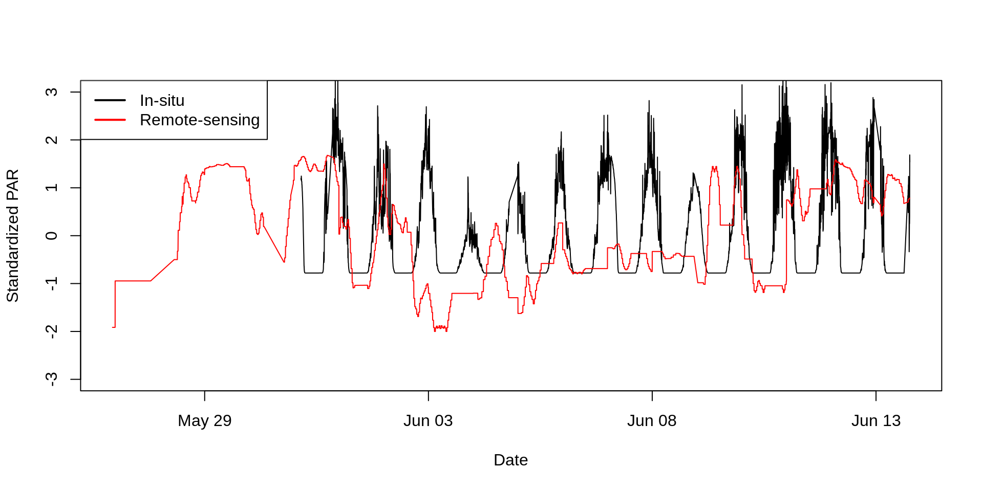

We can see that remote sensing PAR is messy (probably due to factors like cloud cover) compared to the consistent, non-erratic daily fluctiation of in-situ PAR.